1 Department of Environmental Sciences, Western Norway University of Applied Sciences, Sogndal, Norway
2 Department of Computer Science, Electrical Engineering and Mathematical Sciences, Western Norway University of Applied Sciences, Bergen, Norway
Engineering Geology · 2026
Abstract
In this paper, we propose to use causal feature selection to only use the most relevant variables in a surface displacement prediction task on an unstable rock slope. We show that this improves prediction performance across models. Moreover, we show that using a Kolmogorov-Arnold Network (KAN) further enhances the predictive capability while offering superior interpretability. The latter is due to the activation functions the KAN employs, which allow for a more transparent understanding of the model's decision-making process after training without using post-hoc explanation methods such as LIME and SHAP.
Background
Landslides and unstable rock slopes pose significant risks to human lives and infrastructure and have been the subject of extensive research on how to understand the underlying drivers of (surface) displacement processes as well as predicting future displacement. The main challenge is that existing studies focus on either understanding cause-effect relations OR predicting surface displacement, but not both together. Additionally, (complex) neural networks used in most existing studies are difficult to interpret, creating adoption issues for geoscientists who are non-experts in machine learning. Where interpretation is implemented it is often based on post-hoc explanation methods such as LIME and SHAP, which are non-intuitive to interpret and computationally expensive.
Key Ideas
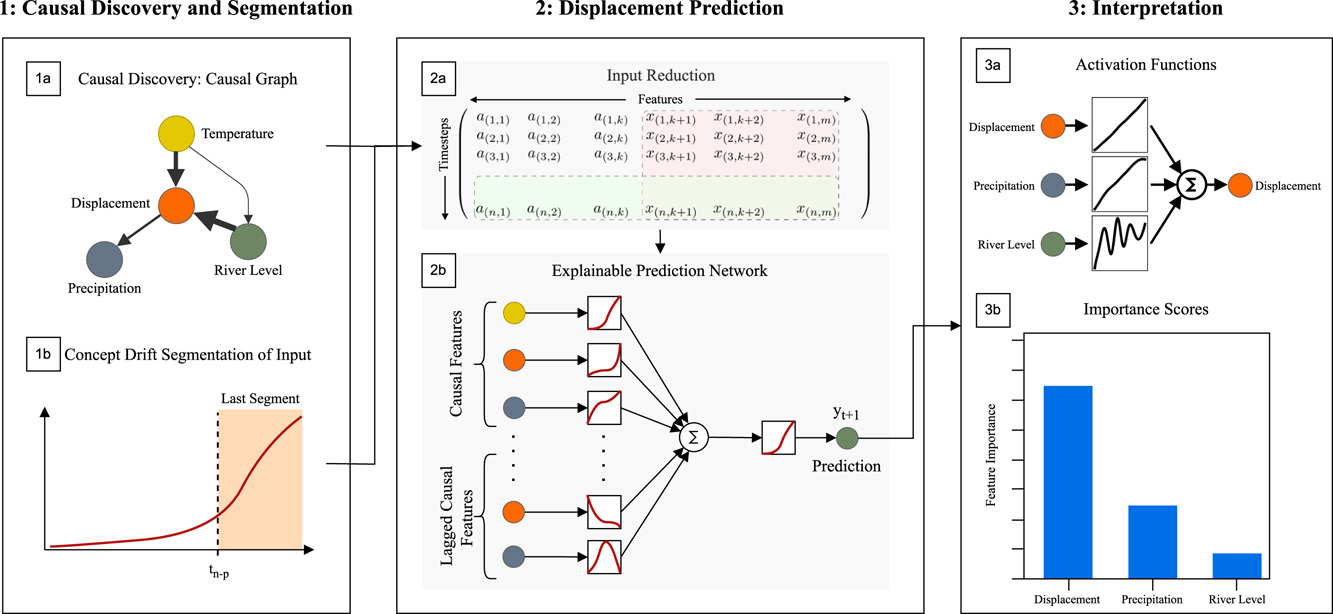
We propose a two step framework:- Module 1: Uses Multi-Window Causal Discovery to identify causal features and segments non-stationary time series (see also the blog post on the MWCD paper)
- Module 2: Performs prediction using only the relevant causal variables as well as the time series only within the last segment according to the Module 1 output. Prediction can be implemented using your favourite model, we employ Kolmogorov-Arnold Networks (KANs), which optimize activation functions rather than connection weights, enabling visualization of learned relationships.
Application
We applied our framework to three different sites with different geological conditions and different displacement characteristics to demonstrate effectiveness and transferability. For each site, we trained the following models:
- Multilayer Perceptron (MLP)
- Long Short-Term Memory (LSTM)
- Gated Recurrent Unit (GRU)
- xLSTM
- Random Forest (RF)
- Extreme Gradient Boosting (XGBoost)
- Mamba
- Kolmogorov-Arnold Network (KAN)
For all models we trained with the data in all four configurations: full data, causal factors only, last segment only, and causal factors within the last segment.
For each model and dataset we optimised the hyperparameters using a grid search with sensible ranges for all parameters.
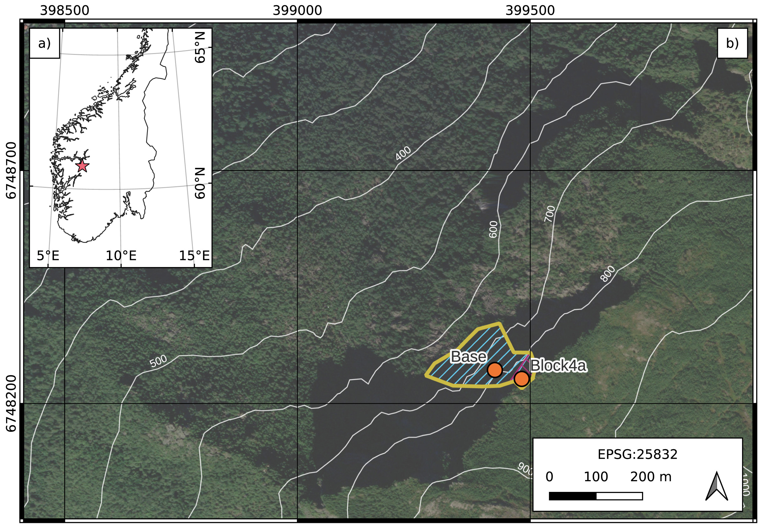
Figure 1 illustrates one of the application areas: Sensor network on a rock section where displacement is being monitored along with precipitation, temperature, soil moisture and infiltration of water into the ground.
For this particular site the MWCD framework helps in identifying the causal relationships and segmenting the time series as shown in Figure 2.
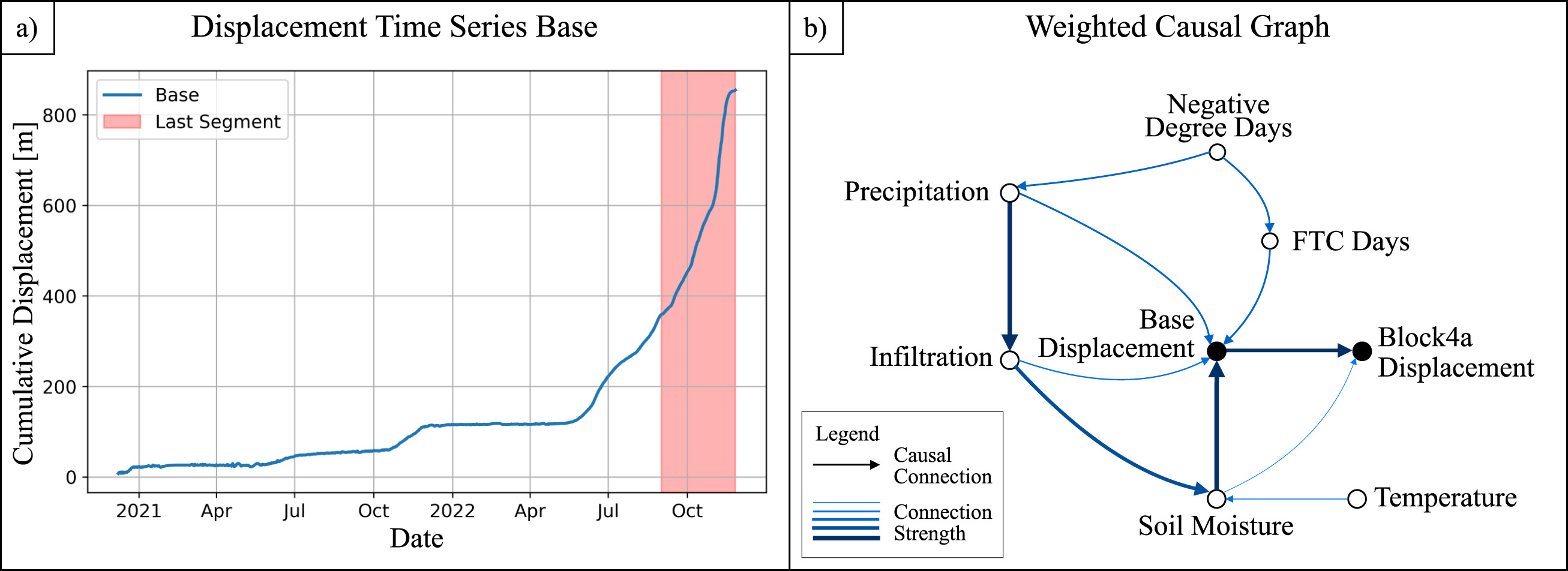
Causal feature selection in this case identifies the most relevant factors influencing Base Displacement as Precipitation, Infiltration, Soil Moisture and Freeze-Thaw Cycles.
The last segment of the time series according to the detected changes in the underlying sample generating process starts in September 2022.
The different models compare as presented in the table below. Notably, the KAN model outperforms all other models when using the Causal inputs only within the last segment of the time series, achieving both lowest RMSE and highest R2 value.
| Model | Baseline | Causal | Last segment | Causal last segment | ||||
|---|---|---|---|---|---|---|---|---|
| RMSE | R2 | RMSE | R2 | RMSE | R2 | RMSE | R2 | |
| MLP | 1.2002 | 0.4084 | 1.0108 | 0.5926 | 1.0058 | 0.5638 | 1.2150 | 0.3198 |
| LSTM | 1.1666 | 0.4540 | 1.5298 | 0.0669 | 1.4829 | 0.0518 | 1.4925 | -0.0112 |
| GRU | 1.4759 | 0.1260 | 1.3884 | 0.2314 | 1.2949 | 0.2591 | 1.3737 | 0.1863 |
| xLSTM | 1.6159 | -0.0597 | 1.4499 | 0.1279 | 1.3624 | 0.1799 | 1.3766 | 0.1396 |
| Random Forest | 1.6977 | -0.1562 | 1.6733 | -0.1363 | 1.4812 | 0.0306 | 1.4845 | 0.0264 |
| XGBoost | 4.4253 | -0.1149 | 4.3631 | -0.0838 | 5.7036 | -0.1416 | 5.5706 | -0.0663 |
| MAMBA | 1.0477 | 0.5597 | 1.4557 | 0.1401 | 1.1816 | 0.3980 | 1.1429 | 0.4229 |
| KAN | 1.2565 | 0.5628 | 1.5123 | 0.6146 | 1.0528 | 0.6036 | 1.0525 | 0.6201 |
Using the causal features and, in this case, also only the last segment improve the predictive performance considerably. It makes intuitively sense to rely only on the factors that actual cause the displacement. Similarly, using only data from the same underlying sample distribution as the prediction horizon improves the model's ability to generalize and make accurate predictions. This is however only the case if the last segment has different displacement characteristics from the others. In the case of relatively constant dispalacement, having more data will be beneficial and thus the whole time series should be used (see presented application case on "Vögelsberg").
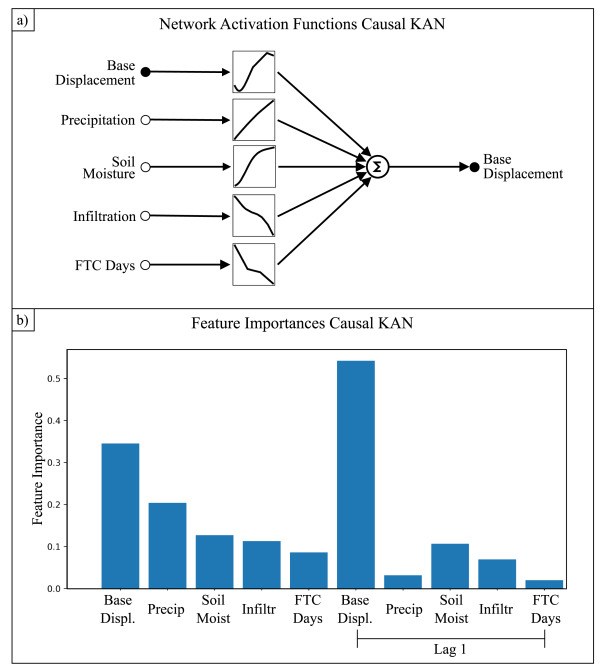
An additional contribution is to visualise the relations the model has learned between the input features and the output. In the case of the KAN model it explains itself through visualisation of the activation functions (Figure 3 here below). When supplied with the feature importance, it offers a useful model explanation that will also help with counterfactual explanations, i.e. what would have been the prediction if certain features had taken different values.
Site comparison
The table below provides an overview over the different sites and the results we obtained for each of them.
| Site name | Stampa | La Clapière | Vögelsberg |
|---|---|---|---|
| Features | Block Displ. Base Displ. Soil Moisture Infiltration Precipitation Temperature NDD Consec. NDDs FTC Consec. FTCs | CLP0 Displ. CLP5 Displ. CLP6 Displ. River Level River Temperature River Conductivity Air Temperature Precipitation NDD Consec. NDDs FTC Consec. FTCs | D_WS_1 Displ. D5_1 Displ. SWVL (1-4) Snowmelt Air Temperature Precipitation NDD Consec. NDDs FTC Consec. FTCs |
| Description | Multiple accelerations | Sharp acceleration | Steady displacement |
| Causal Graph | Four incoming target connections | Three incoming target connections | Two incoming target connections |
| Best Model | KAN with Causal Last Segment | KAN with Causal Last Segment | KAN and MLP with Causal factors only (over full timespan) |
Conclusion
The proposed method outperforms almost all recent machine learning approaches in prediction accuracy while offering easy interpretability. KAN-based models consistently achieved the best performance when using causal features, with significant RMSE reductions (up to 54% improvement) .
Citation
@article{SCHILD2026109044,
		title = {Explainable surface displacement prediction using causal feature selection and Kolmogorov-Arnold Networks},
		journal = {Engineering Geology},
		volume = {373},
		pages = {109044},
		year = {2026},
		issn = {0013-7952},
		doi = {https://doi.org/10.1016/j.enggeo.2026.109044},
		url = {https://www.sciencedirect.com/science/article/pii/S001379522600503X},
		author = {Lukas Schild and Thomas Scheiber and Paula Snook and Alexander Maschler and Reza Arghandeh},
}